Analytical vs. Preparative Chromatography Explained
Analytical and preparative chromatography rest on the same separation principle but serve different goals: one is run to obtain information, the other to obtain purified material. Because the goals differ, the hardware and methods differ substantially — and the difference runs all the way down to the trade-offs at the heart of preparative work.
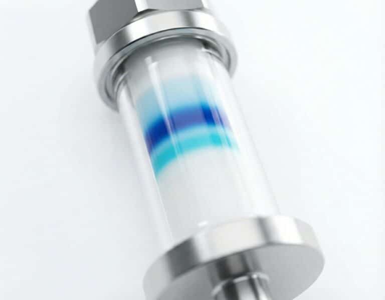
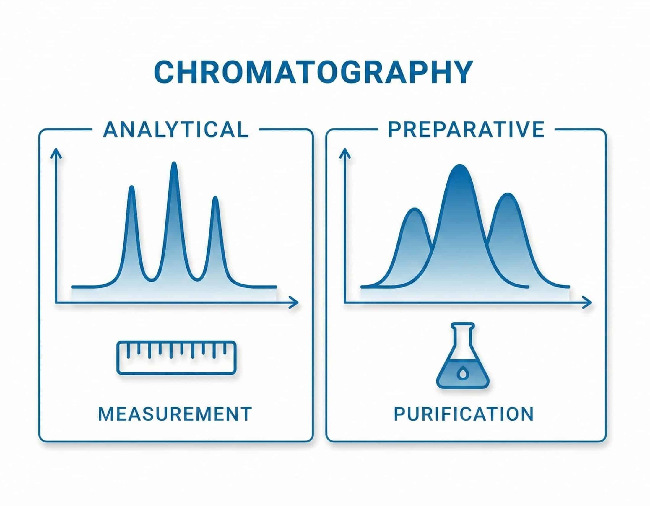
Part I introduced chromatography as a single principle: a mixture flows through a medium, its components travel at different speeds, and they separate. Every run is performed for one of two reasons: to analyze a sample — identifying and quantifying its components — or to purify it, isolating a target compound in usable quantity. This article examines the second, preparative chromatography, and how the goal of collecting material shapes its columns, instruments, and methods.
Although analytical and preparative chromatography rely on the same principle of separation and use the same broad component types — columns, pumps, resins, detectors — the instruments themselves diverge. One built to detect trace amounts and one built to collect kilograms differ in column dimensions, particle size, flow rate, detector design, and materials of construction.
Analytical chromatography is about information; preparative chromatography is about material.

1. Two Purposes, One Principle: Information vs. Material
Analytical and preparative chromatography are distinguished by what remains of value once the run ends: for analytical work, the data; for preparative work, the purified material itself.
Analytical chromatography produces a chromatogram and the data drawn from it; the sample is consumed in the measurement and passes to waste after the detector. It answers what a sample contains, how much of each component is present, and which trace impurities or degradation products are detectable. Method development therefore optimizes resolution (clean separation between peaks), sensitivity (detection of small amounts), and sharp, symmetrical peaks for accurate integration.

Preparative chromatography reverses this priority. The data serve only as a means; the product is physical material — a purified target compound collected in usable quantity. The same separation operates across a wide range of scales:
- Discovery (milligrams) Isolating candidate compounds or natural products to the purity required for biological screening and structure confirmation.
- Development (grams) Purifying proteins, peptides, and oligonucleotides to the quality required for toxicology studies and early clinical trials.
- Manufacturing (kilograms and beyond) Polishing APIs, biologics, vaccines, and insulin to final specification.

A Simple Analogy
An analytical run is like photographing an orchard to count and identify the fruit; a preparative run is the harvest. One ends in knowledge, the other in a crate of apples.
2. What Is Preparative Chromatography?
Preparative chromatography is liquid chromatography run to prepare (collect) purified material rather than to measure it.
A run becomes preparative the moment fractions containing the target compound are deliberately collected for downstream use — whether tens of milligrams for a research assay or kilograms for a production batch.
One piece of hardware defines the category: the fraction collector. It distinguishes two flow paths:
Analytical
Column → Detector → Waste

Preparative
Column → Detector → Fraction Collector

Without a means to divert and capture the target peak, no column — however large — performs true preparative work. (Section 3 returns to how the collector decides what to keep.)
Because the goal is material, success is measured differently. Three performance metrics describe any preparative process:
- Purity How clean the collected product is.
- Yield (recovery) The fraction of loaded target compound that is kept.
- Throughput How quickly it is produced.
Which of these pull against one another depends on the step; balancing them deliberately is the central skill of preparative chromatography, and the subject of Section 7.
3. Same Principle, Different Machine
Because intent drives design, almost every component is sized and built differently once the goal shifts from measurement to collection.
Scale and Sample Load
Scale is the most visible difference. Analytical systems handle trace amounts — nanograms to micrograms, at injection volumes of roughly 1–10 µL. Preparative systems handle milligrams to kilograms, at injection volumes from milliliters to hundreds of liters at process scale. Most other differences follow from this gap.
Columns and Particle Size
To hold more material, a preparative column can be far wider than an analytical one — from tens of millimeters up to a meter or more at production scale. Width scales with the amount of material, though: in process development the column narrows to analytical dimensions, down to 4.6 mm ID on a preparative system, or smaller still on an analytical one (Section 4). What consistently marks a column as preparative is therefore not its width but its packing — larger particles, typically 10–50 µm, against the sub-2–5 µm of analytical HPLC and UHPLC. Smaller particles deliver higher efficiency and resolution at the cost of higher backpressure, as the next subsection explains.
Flow, Velocity, and Column Volumes
Three variables recur throughout preparative work, and two of them are defined to be independent of column size — the property that lets a method transfer from a small column to a large one unchanged.
- Volumetric flow rate (mL/min) The volume of mobile phase the pump delivers per minute. It is set on the pump and scales with the column’s cross-sectional area.
- Linear velocity (e.g., cm/h) The speed at which the mobile phase travels through the packed bed — approximately the volumetric flow rate divided by the column’s cross-sectional area. Two columns of different diameter share the same linear velocity when their volumetric flow rates are scaled in proportion to their areas. Linear velocity, not volumetric flow rate, governs both the separation and the backpressure.
- Column volume (CV) The total volume of the packed bed — the resin particles plus the liquid filling the spaces between and within them — used as a size-independent unit. “Wash with 3 CV” or “run the gradient over 20 CV” denotes the same operation on a 4.6 mm column and on a 50 mm one.
- Gradient slope (%B per CV) The rate of change of mobile-phase strength. Expressed per column volume rather than per minute, it is also size-independent: the same slope produces the same separation at any column diameter.
Describing a method in linear velocity and column volumes, rather than mL/min and minutes, is what makes linear scale-up possible (Section 6).
Flow Rate and Pressure
To keep batch times reasonable, preparative volumetric flow rates run an order of magnitude above analytical ones — tens to hundreds of mL/min at lab scale, liters per minute in production, against 0.1–5 mL/min for analytical work. The effect on pressure is widely misunderstood; three points clarify it:
- A wider column does not by itself raise pressure At a given linear velocity, column diameter has essentially no effect on backpressure; the wider column simply carries more volume.
- Particle size is the dominant lever Backpressure scales roughly with the inverse square of particle diameter: halving the particle size quadruples the pressure. Preparative columns therefore use larger particles, which permit high volumetric flow rates without exceeding the pressure limit of the bed or hardware.
- Linear velocity and viscosity matter too Pressure also rises with linear velocity, mobile-phase viscosity, and bed length — but particle size has the steepest effect.
The result is a pressure gap between analytical and preparative work, driven mainly by particle size:
- Analytical HPLC: commonly up to ~400 bar; UHPLC up to ~1000 bar or more, because sub-2 µm particles demand it.
- Preparative HPLC: highly variable — many lab systems and their flow paths are rated to around 100 bar, while dedicated high-pressure prep systems run well above that.
- FPLC: low pressure by design — often well under 50 bar, and only a few bar for the softest agarose resins.
Why not, then, build a large system rated to 400–1000 bar and keep the fine particles? Because structural force does not scale up gracefully. The total force a column must contain is its cross-sectional area multiplied by the pressure, and that area grows with the square of the column’s width. So holding the same pressure rating while widening a column from 4.6 mm to 50 mm raises the total force on end frits, seals, and walls more than a hundredfold (roughly 118 times), and a column tens of centimeters across faces a far larger load still — a pressure trivial to contain in an analytical tube becomes a serious mechanical and safety hazard at scale. The packing is also vulnerable: a tall bed of fine particles can compress or fracture under a steep pressure drop, causing the bed to collapse and destroying the efficiency the small particles were chosen to provide. The practical, economical solution is to remove the need for the pressure entirely by using larger particles.
In summary, the wider column carries more volume and the larger particles keep pressure within manageable limits. (As Section 4 shows, that ~100 bar ceiling is where the boundary between preparative and analytical hardware begins to blur.)

Detection
Detection is easily overlooked. Analytical detectors are optimized for sensitivity — detecting the faintest trace. Preparative detectors face the opposite problem: the eluting product is concentrated enough to saturate an ordinary detector immediately. UV absorbance follows the Beer–Lambert relationship — absorbance rises with both concentration and the optical path length of the flow cell — so preparative systems use very short path-length cells, or monitor at a wavelength of weak absorbance, to keep the signal on-scale. The detector need not quantify trace impurities; it need only track the target peak accurately enough to trigger the fraction collector.
System Materials: HPLC vs. FPLC
The materials of construction depend on what is being purified. The broad division is preparative HPLC for robust small molecules and FPLC for sensitive biomolecules:
Preparative HPLC
Essentially analytical HPLC scaled up: stainless-steel systems, organic solvents, high-pressure pumps. Suited to small, robust molecules that tolerate these conditions.
FPLC (Fast Protein Liquid Chromatography)
Lower pressures and biocompatible materials — glass, titanium, PEEK — for proteins and other large biomolecules that need gentler handling.
Biomolecules require the gentler FPLC environment for three reasons:
- Proteins and other large biomolecules can denature under high pressure and organic solvents.
- The soft, agarose-based resins used to separate them compress under high pressure, requiring low-pressure operation.
- The high-salt aqueous buffers common in biomolecule work — chloride especially — corrode stainless steel, which FPLC therefore avoids.
The division is not absolute — peptides and oligonucleotides, for example, are often purified by reversed-phase HPLC — but as a general rule, robust small molecules use HPLC and sensitive biomolecules use FPLC.
The Fraction Collector, Revisited
The fraction collector captures the target peak using one or more triggers: a time window; an absorbance threshold (collecting while the signal exceeds a set level); slope or peak detection (starting at the leading edge, stopping at the trailing edge); or, increasingly in discovery work, a mass-spectrometry trigger that collects only when the target’s mass is detected. The essential point — and the reason an overloaded preparative chromatogram still yields pure product — is that the collector need not keep the whole peak. Where the target peak overlaps impurities, the operator collects only the central, purest portion, the center cut, and diverts the overlapping shoulders to waste or to a vessel for reprocessing. This is the practical lever behind the purity–yield trade-off, and The Polishing Trade-Off is built around it.

4. Where Analytical and Preparative Overlap
The contrast above describes a spectrum, not a sharp divide. Analytical and preparative denote a run’s purpose and scale, not mutually exclusive categories of hardware, and in the middle ground the two share equipment freely. The practical consequence is that a separate analytical-scale instrument is usually not required to develop a preparative method.
The boundary is set mainly by pressure and particle size, not by column diameter or flow rate. Most of the apparent overlap follows from this.
Shared Resins and Columns at the Semi-Prep Scale
Semi-preparative resins and columns sit squarely in this overlap. A semi-prep column runs on an analytical instrument for a small isolation, or on a small preparative system for a larger one — the same resin and dimensions serve both. The question is which instrument the column is run on, not which category it belongs to.
Small Prep Systems Can Run Analytical-Dimension Columns
For process development this is the key point. A compact lab-scale preparative system — such as ChromaCon’s Contichrom CUBE — can run a narrow, analytical-dimension column (down to 4.6 mm ID) packed with the larger particles used at scale. This is often preferable to scouting on a true analytical instrument:
- No particle-size mismatch UHPLC’s sub-2 µm particles have no preparative equivalent, so a UHPLC method cannot be scaled in particle size. Developing on the preparative particle size from the start makes scale-up more reliable.
- One platform, start to finish The same system used to scout the method can run it at small production scale, removing an instrument-to-instrument transfer.
Thus “develop small, then scale up” refers to working at small column dimensions and loads, not to owning a dedicated analytical system.
The Hidden Hurdle: Extra-Column Volume
While a lab-scale prep system can pump at analytical flow rates, there is a catch: extra-column volume. Standard preparative systems have wide tubing and large flow cells designed for high flow rates. If a narrow 4.6 mm column is attached, the relatively huge volume of the system’s tubing will mix and dilute the separated peaks after they exit the column, destroying resolution before it reaches the detector. Small-scale preparative systems designed specifically for method development (such as ChromaCon’s Contichrom CUBE) use specialized flow paths to prevent this dispersion.
Low Flow Rates, Accurate Gradients
A preparative pump is sometimes assumed too coarse to form the precise gradients an analytical-dimension column needs at low flow. In practice, prep systems with pump flow rates below roughly 40 mL/min can form accurate gradients at the low flow rates such a column requires — down to about 4.6 mm ID, matching an analytical system for gradient fidelity. Below that diameter the required flow rates fall too low for a preparative pump to meter the gradient accurately.
The One Real Limit — and Its Exception
What a typical prep system often cannot do is run very small particles, for reasons of pressure:
- Particles below ~10 µm typically require more than ~100 bar to drive the mobile phase through them at useful flow rates.
- Many preparative systems — pump heads, valves, seals, flow-path materials — are rated to around 100 bar, so sub-10 µm particles cannot be used on that hardware.
This limit has an exception. High-pressure preparative systems run small particles at preparative flow rates, combining analytical-grade resolution with material collection — precisely what impurity isolation demands: collecting a closely eluting impurity in usable quantity while retaining the resolution needed to separate it from the main peak.
Choosing among FPLC, MPLC, and preparative HPLC for a given molecule — and matching the system to its buffers, resins, and scale — is a larger decision, covered in a dedicated guide to system selection. The point here is narrower: the analytical-to-preparative boundary is set by pressure and particle size, not by column diameter or flow rate, so small-scale method development rarely requires a separate analytical instrument.
5. Analytical and Preparative at a Glance
| Feature | Analytical Chromatography | Preparative Chromatography |
|---|---|---|
| Primary goal | Information (qualitative + quantitative) | Isolation and purification of the target compound |
| Desired outcome | Data (a chromatogram) | Purified physical product |
| Optimization focus | Resolution, sensitivity, peak shape | Purity, yield (recovery), throughput |
| Amount processed | Trace (ng–µg) | Milligrams to kilograms |
| Injection volume | ~1–10 µL | mL to hundreds of L |
| Column inner diameter | Narrow (≤ 4.6 mm) | Varies with scale: ~4.6 mm (dev) to >1 m (production) |
| Particle size | Small (sub-2–5 µm) | Larger (~10–50 µm) |
| Flow rate | Low (~0.1–5 mL/min) | High (~10 mL/min to L/min) |
| Backpressure | Higher (small particles): HPLC to ~400 bar, UHPLC ~1000 bar+ | Lower (larger particles): many systems ~100 bar, high-pressure prep above |
| Column loading | Kept low to preserve resolution | Deliberately overloaded for throughput |
| Detection | Maximize sensitivity | Avoid saturation (short path-length cells) |
| Fraction collector | Usually absent (sample to waste) | Essential for product recovery |
| Typical peak shape | Sharp, near-Gaussian | Broader, often asymmetric (“shark-fin”) |
6. Why Small-Scale Methods Always Come First
A preparative campaign almost always begins at small scale. Before valuable material is committed to a large column, the target compound’s behavior must be established — which solvents, pH, buffers, and gradients best separate it from its impurities. Small-scale work suits this scouting because it is fast (small columns equilibrate quickly), economical (minimal sample and solvent), and low-risk (a failed experiment wastes almost nothing).
As Section 4 noted, “small-scale” here means small columns and loads, not necessarily a dedicated analytical instrument. Scouting can run on an analytical HPLC, or on a small preparative system using an analytical-dimension column packed with the intended scale-up particle size. The conditions found are then transferred upward by linear scale-up, whose principle is to increase column capacity without changing the separation itself:
Held constant
Stationary-phase chemistry, particle size, column length (bed height), linear velocity, mobile phase, and gradient slope (in column volumes).
Scaled up in proportion
Column cross-sectional area (its diameter), volumetric flow rate, and sample load — all increased together.
Because the separation is expressed in the size-independent terms from Section 3 — linear velocity and column volumes — a method optimized on a 4.6 mm column can in principle be reproduced on a 50 mm column running the same chemistry at a proportionally higher flow rate. Small-scale chromatography is where the method is discovered; preparative chromatography is where it is executed at scale.
7. The Trade-Offs at the Heart of Preparative Chromatography
One further difference is a choice rather than a component: preparative chromatography is run under conditions analytical work avoids. To produce material at a useful rate, far more sample is loaded, and the sharp, symmetrical peaks of analytical separation give way to the broader, asymmetric, often overlapping peaks characteristic of an overloaded column.
A purification is rarely a single column. It usually runs in stages: a capture step first — extracting the target compound from a large, crude feed to concentrate it and remove the bulk of the contaminants — followed by one or more polishing steps that remove the last, closely related impurities to reach final specification. Both are judged on the same three measures, but they place different ones in tension.
Capture
Purity is set largely by the feed and the wash, and yield is held high by design — the column is loaded below the point of product breakthrough. The remaining trade-off is between using the expensive resin fully and running the step fast. This is dictated by residence time: pushing the mobile phase too quickly leaves target molecules with insufficient time to diffuse into the resin pores, significantly lowering the column’s dynamic binding capacity.
Polishing
The target compound is already largely pure; the task is separating it from impurities that elute close by. Purity and yield oppose each other directly — a narrow center cut protects purity but discards product, a wider one recovers more but admits impurity — with throughput pressing on both.
Both compromises — trading resin utilization for speed in capture, and trading yield for purity in polishing — were long treated as unyielding laws of traditional batch chromatography.
Breaking the Batch Constraints: Continuous, multi-column chromatography fundamentally rewrites these rules. By structurally linking columns in series, a second column can automatically capture the product breakthrough or overlapping peak shoulders that a single batch column is forced to discard.
The next two articles in this series explore these advanced architectures in the exact order a process encounters them: Part III: The Capture Trade-Off (CaptureSMB), followed by Part IV: The Polishing Trade-Off (MCSGP).

8. Key Terms Introduced in This Article
| Term | Definition |
|---|---|
| Target compound | The specific molecule you intend to isolate from a mixture. |
| Preparative chromatography | Chromatography run to collect purified material rather than to measure it. |
| Fraction collector | The hardware that diverts and captures the eluent containing the target peak. |
| Yield (recovery) | The percentage of loaded target compound that ends up in the collected product (Mass Out / Mass In). |
| Throughput | The amount of purified product made per unit time. |
| Center cut | The central, purest portion of an overlapping peak, collected to maximize purity. |
| Volumetric flow rate | The volume of mobile phase delivered per unit time (mL/min); set on the pump and scaled with column cross-section. |
| Linear velocity | How fast the mobile phase travels through the packed bed; the size-independent driver of separation and backpressure. |
| Column volume (CV) | The volume occupied by the packed column, used as a size-independent unit for washes and gradients. |
| Gradient slope | How fast the mobile-phase strength changes; expressed per column volume (%B/CV) to stay independent of column size. |
| FPLC (Fast Protein Liquid Chromatography) | Low-pressure LC on biocompatible systems, designed for proteins and other biomolecules. |
| Semi-preparative | Small-scale purification (roughly microgram to low-milligram) that bridges analytical and full preparative work. |
| Linear scale-up | Transferring a method to a larger column by scaling cross-sectional area, flow, and load while holding the separation conditions constant. |
9. Frequently Asked Questions
Yes. Both rely on the mechanism described in Part I: components partition differently between the stationary and mobile phases and separate as they travel through the column. The difference is intent — information versus material — not the underlying physics.
Generally no. Analytical systems are not built for the large injection volumes and high flow rates preparative work requires, and they usually lack a fraction collector. An analytical instrument can sometimes manage very small semi-preparative isolations (microgram to low-milligram), but not the milligram-to-kilogram scale that defines preparative chromatography.
No. Method development requires small column dimensions and loads, not a dedicated analytical instrument. A compact preparative system (for example, ChromaCon’s Contichrom CUBE) can run an analytical-dimension column — down to 4.6 mm ID — packed with the larger particles used at scale. Developing on that preparative particle size is often better than scouting on a UHPLC, whose sub-2 µm particles have no preparative equivalent and cannot be scaled in particle size. Prep systems with pump flow rates below about 40 mL/min also form accurate gradients at the low flow rates such a column requires, so gradient fidelity is not a barrier — though 4.6 mm ID is about the lower limit, since columns narrower than that require flow rates too low for a preparative pump to meter the gradient accurately, and extra-column volume typically causes massive dispersion.
It depends on the system’s pressure rating. Particles below ~10 µm require more than ~100 bar to drive flow, and many prep systems — pumps, valves, seals, flow-path materials — are rated to around 100 bar, which excludes those particles. High-pressure preparative systems are the exception, running small particles at preparative flow rates and so combining analytical-grade resolution with material collection — exactly what impurity isolation requires: collecting a closely eluting impurity in usable quantity while keeping the resolution needed to separate it from the main peak.
Because the column is deliberately overloaded. At high load, standard chromatography is governed by Langmuir isotherms, meaning most compounds form an asymmetric peak with a sharply rising front edge and a long, drawn-out tail (the “shark-fin” shape) while neighboring peaks broaden and overlap. (Pronounced fronting — a gradual leading edge ending in a sharp drop — is less common, arising from unusual adsorption behavior or from injecting the sample in a solvent stronger than the mobile phase.) This does not indicate a failed run: the fraction collector simply isolates the clean center of the target peak. The Polishing Trade-Off explains the underlying physics.
The fraction collector takes only the central, purest part of the target peak — the center cut. The shoulders, where the target compound co-elutes with impurities, go to waste or are collected separately for reprocessing. This secures high purity at the cost of some yield — exactly the trade-off explored in The Polishing Trade-Off.
To keep backpressure manageable. Preparative work requires high volumetric flow rates, and pressure rises steeply as particle size shrinks (roughly with the inverse square of particle diameter). Larger particles let the system run fast without exceeding the pressure limits of the column or hardware, while still resolving the target well enough to collect it. At a given linear velocity the wider column itself adds no pressure; particle size is what matters.
Because structural force does not scale up gracefully. The same pressure acts over a far larger cross-section in a wide column, so the total force on seals, frits, and walls climbs proportionally with area. A pressure rating easily contained in a 4.6 mm tube creates over 100 times more total structural force in a 50 mm column. A massive bed of fine particles can also compress or fracture under a steep pressure drop, ruining the efficiency the small particles were chosen to provide. The safer, economical answer is to remove the need for extreme pressure by using larger particles.
Proteins and other biomolecules generally require gentle, aqueous, non-denaturing conditions; the high pressures and organic solvents of HPLC can damage them, and the soft resins used to separate them compress under pressure. FPLC runs at lower pressure, uses biocompatible materials, and tolerates the high-salt buffers these separations require. Small molecules are usually robust enough for high-pressure, stainless-steel HPLC with organic solvents. (Peptides and oligonucleotides are a common middle ground, often purified by reversed-phase HPLC.)
No. “Preparative” describes the purpose, not the size. A bench purification of a few tens of milligrams is preparative if its aim is to collect material for downstream use.
Almost always no. GC handles small amounts of volatile compounds and is inefficient for collecting bulk material. “Preparative chromatography” nearly always denotes a liquid technique — preparative HPLC, FPLC, or another form of prep LC.
Balancing the three competing goals — purity, yield, and throughput — for a given molecule and stage of development. There is no universally best method, only the best compromise for the task. That balance is the subject of The Polishing Trade-Off.